Project research MIT PRIMES 2026
A signal from Saturn.
A closer look at its rings.
Cassini sent radio waves through Saturn’s rings. Our team studies the mathematics that could help recover finer detail from the signals that reached Earth.
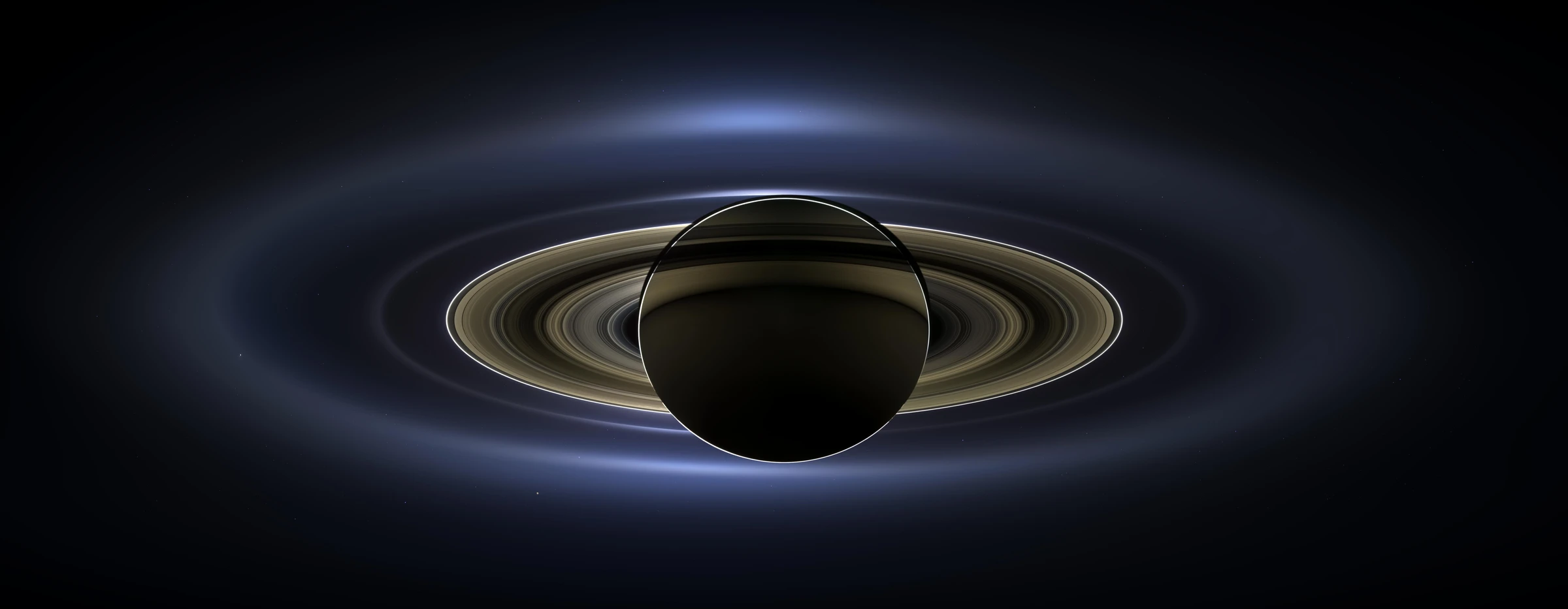 See the original image
 01 / Where the question begins
The rings leave a trace.
How do we read it?
As a radio signal passes through the rings, its strength and phase change. Those changes carry information about the material it crossed.
Recovering fine structure also means accounting for diffraction: waves travelling along nearby paths interfere. Our project begins with the calculation that connects this signal to the rings.
How Cassini used radio signals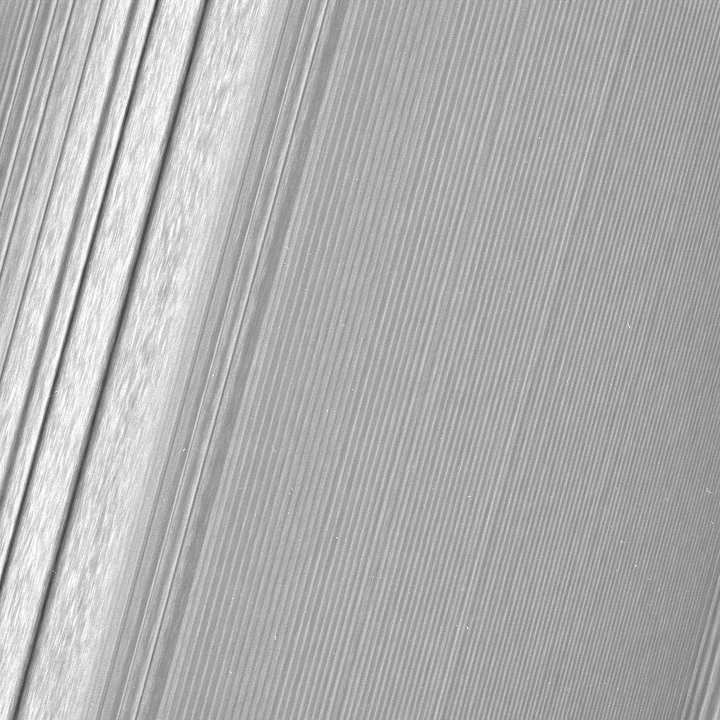 Look closer
 What does the radio observation look like?Open a real Cassini profile and follow it into the Data explorer.
Our explorer contains six calibrated ring profiles from the NASA Planetary Data System. They retain diffraction effects and provide a starting point for reconstruction.
The mathematical question
One root can hide
another branch.
A stationary-phase calculation focuses on angles where the phase stops changing. One starting guess can find one such angle and miss others. Near a fold, two branches approach each other and turn.
A stationary angle is a root of the phase derivative at ring radius .
How do we find the relevant branches, keep their identities, and decide when the approximation needs more care?
02 / Following the signal’s structure
Find the roots.
Keep the story of each one.
A stationary root is one place where the signal’s phase stops changing with angle. The challenge is to find all the relevant roots, then understand which branch each belongs to as we move across the rings.
- Find
Give each root a starting point.
At one ring radius, the stationary equation can have several solutions. Padé approximation and adaptive least-squares fits provide candidates for the roots that are harder to find.
Carry forwardA set of candidate roots
- Follow
Stay with the curve as it turns.
As the radius changes, the roots move. Pseudo-arclength continuation follows the branch itself, including near a fold, instead of treating every radius as a fresh search.
Carry forwardA connected branch to follow
- Check
Ask the original equation again.
Interpolation returns the candidates to the data grid. Halley’s method then refines them on the original equation, while residual and sampling checks test whether they should be accepted.
Carry forwardRefined roots with numerical checks
A root also needs an identity.
A numerical solver may return the same roots in a different order. One-to-one matching reconnects them using circular angle distance, preserving a record of each branch’s phase, curvature, amplitude, and status.
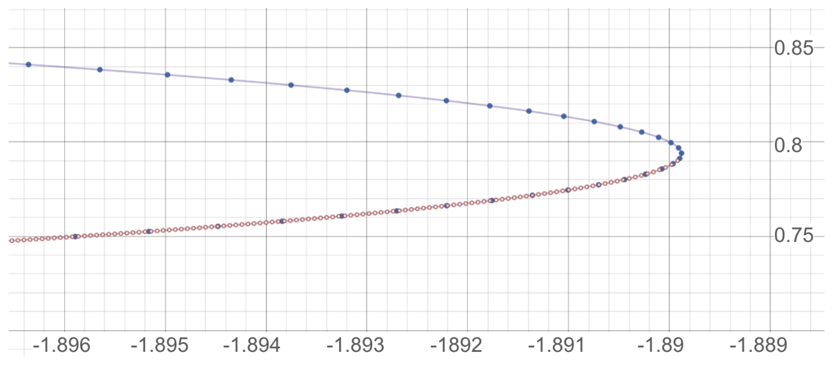
A closer lookFollow a worked branch.See the team’s continuation experiment at the point where the curve turns.
From the working manuscript
The method follows the turn.
The blue continuation points move around the fold. Red PCHIP points return one branch to a regular grid; the purple curve provides the marching-squares comparison.
Try a simpler model yourself
A teaching model
When two paths become one.
Here, a simple cubic makes the geometry visible.
Three roots, three paths.
The vertical line meets three branches. Each intersection is a solution at this parameter; following a branch preserves the connection between nearby solutions.
Root values: -1.5321 · -0.3473 · 1.8794
The equations behind the three steps
The team seeks stationary angles: places where the phase stops changing with angle.
01 / Initial candidates
A simpler function to solve.
At a fixed radius, numerator roots supply candidates. Candidates associated with denominator poles are excluded. Adaptive fitting concentrates on the extra pair after the stable root is found.
02 / Continuation
A step along the branch.
With , the second constraint chooses a step along the current tangent. PCHIP interpolation then returns the solutions to regular radii.
03 / Refinement
A correction on the original function.
Functions and angle derivatives are evaluated at the current candidate, at a fixed radius. A small change in the candidate is not sufficient: the equation residual must also be checked.
Working manuscript, §3.1–3.2, pp. 10–17.
Finding the right roots is only part of the problem. Near a fold, even accurate roots can give a poor stationary-phase approximation. The next question is when to change the way we evaluate the signal.
03 / The evidence
One difficult point.
A different calculation.
Follow one example, then open the checks that support it.
Consider a point just 0.001 km from the fold. The stationary roots are already correct, but treating their contributions separately gives a large error. Our next decision is about how to evaluate the integral.
This example tests a local angular contribution in a scalar geometry informed by Rev 133. The percentages compare numerical evaluations with an independent reference; they are not errors in a reconstructed ring profile.
Here the phase gap passes the preset rule, so the evaluator uses Simpson quadrature. The difference comes from that extra calculation, not from changing root labels.
Move farther from the fold Choose one of eight reported offsets, in km.
Across the full tested grid
A local improvement.
A measured trade-off.
- Largest symmetric error
- 59.5629%→2.2872%
- Fewer direct integrand samples than quadrature everywhere
- 37.5%
The rule chooses quadrature at 5 of 8 offsets. It reduces sampling work compared with integrating at every offset; it does not establish a runtime speed-up or a 1% error guarantee.
Inspect all eight results & experiment conditions
| Offset (km) | SPA | + labels | + flags | Switched | Evaluator |
|---|---|---|---|---|---|
| 0.001 | 59.5629 | 59.5629 | 59.5629 | 2.01e-10 | Simpson |
| 0.003 | 49.6822 | 49.6822 | 49.6822 | 2.17e-10 | Simpson |
| 0.01 | 36.5413 | 36.5413 | 36.5413 | 2.01e-10 | Simpson |
| 0.03 | 22.1027 | 22.1027 | 22.1027 | 8.67e-11 | Simpson |
| 0.1 | 6.2333 | 6.2333 | 6.2333 | 8.00e-11 | Simpson |
| 0.3 | 2.2872 | 2.2872 | 2.2872 | 2.2872 | SPA |
| 1 | 0.2756 | 0.2756 | 0.2756 | 0.2756 | SPA |
| 3 | 0.0242 | 0.0242 | 0.0242 | 0.0242 | SPA |
Error definition. Both methods are compared with the same independent reference:
Sampling work. 81,925 direct integrand samples plus 6 saddle evaluations, versus 131,080 integrand samples for quadrature at all eight offsets. Each selected quadrature uses 16,385 Simpson samples. The hybrid requires more work than ordinary SPA.
Independent reference. Adaptive Gauss–Kronrod, checked against 131,073-point Simpson and trapezoid calculations. A common taper is 1 within 0.4° of the fold angle and 0 beyond 0.8°. The threshold was fixed before this comparison. Small quadrature discrepancies do not establish equally small physical uncertainty.
Fixed scalar geometry.
The manuscript cites RSS_2010_170_X34_E_GEO. That geometry product differs from the X43_E_DLP_500M profile available for Rev 133 in the data explorer. The scalar azimuth-to-vector coordinate conversion has not been independently verified.
Two checks behind the result.
Open either experiment to follow the reasoning.
Check the geometryAre the roots really meeting at a fold?A predicted separation law meets independently solved roots.
A disappearing track is not enough to identify a fold. We checked the phase derivatives, counted the nearby roots on each side, and compared their separation with the local prediction.
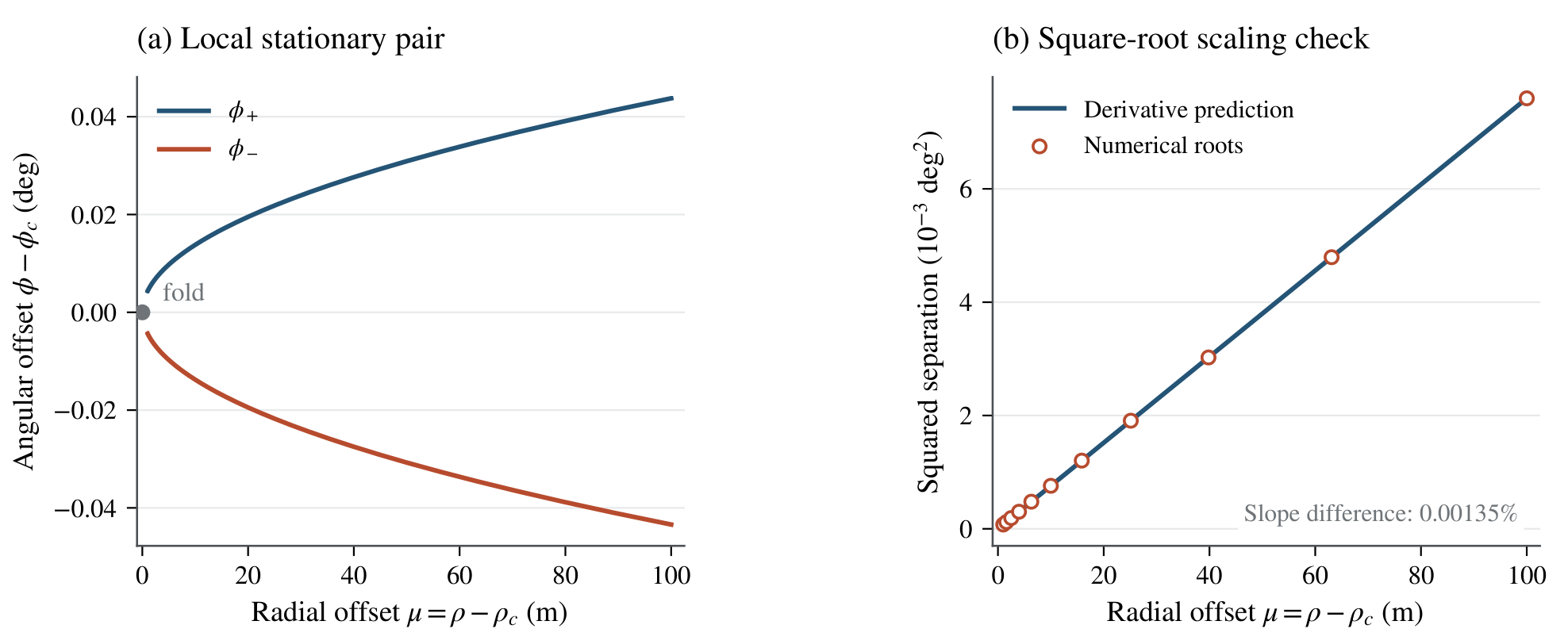
Recomputed location
Squared separation law
- Predicted slope
- 0.07598542
- Measured slope
- 0.07598439
0.001345% reported relative difference
The close agreement supports a local fold in the stated scalar convention. The generic derivative conditions are:
Derivative values & geometry
Reported derivative values use kilometres and radians:
The two displayed slopes are rounded; the relative difference is the manuscript’s reported value. These summary values do not supply a measured root trajectory.
Fixed scalar geometry.
The manuscript cites RSS_2010_170_X34_E_GEO. That geometry product differs from the X43_E_DLP_500M profile available for Rev 133 in the data explorer. The scalar azimuth-to-vector coordinate conversion has not been independently verified.
Team manuscript · Table 2, pp. 18–19
Check the trackingDoes each root keep its identity?Separate a better association from a better integral.
Two nearby roots can both choose the same predecessor if each makes an independent nearest-neighbour match. A one-to-one assignment resolves that competition within a fixed distance gate.
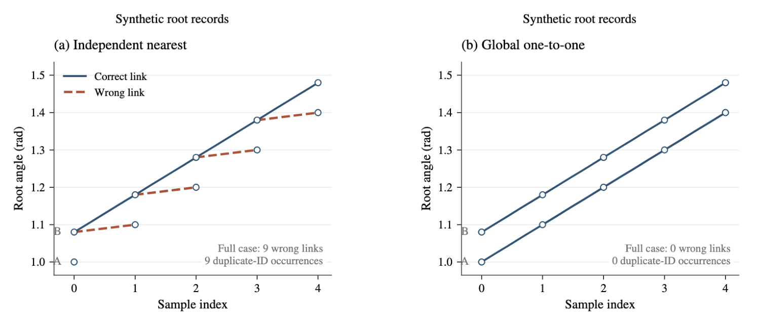
and 9 false unmatched-predecessor flags
and 0 false unmatched-predecessor flags
This improves which root is linked to which. Relabelling the same roots changes their complex sum by at most , at rounding scale. The local-integral improvement above requires the additional integration step.
| Case | Independent matching | One-to-one assignment | Assignment + prediction |
|---|---|---|---|
| Ordinary motion | Passed | Passed | Passed |
| Periodic seam | Passed | Passed | Passed |
| Isolated appearance / disappearance | Passed | Passed | Passed |
| Close parallel tracks | 9 wrong links; 9 false flags | 0 wrong links; 0 false flags | 0 wrong links; 0 false flags |
| Motion beyond the gate | 3 identities lost | 3 identities lost | 3 identities lost |
Prediction made no further improvement in these five cases. When motion exceeded the gate, all methods lost three identities—a case that calls for finer sampling or a recovery step.
How the matching comparison works
Every method receives identical candidate roots. Known identities are used only to assess the links; the random seed changes root order. Assignment first maximizes links within the gate, then minimizes total squared circular distance.
The test evaluates association between samples, not ring-profile reconstruction. An unmatched root can be a missed solution; it does not establish a physical merger.
Team manuscript · §4, pp. 17–18
Reported evidence from our team’s working manuscript, §§4–6, pp. 17–20. The controls explore those results; the website does not rerun the research solver.
04 / The people behind the work
Different pieces.
One shared problem.
The project brings together root finding, continuation, and reliability checks. Each part gives the next one something it can use.
Finding starting points
Yutong Zhao
Worked on Padé approximation and adaptive least-squares methods to locate candidate stationary roots.
Following the branches
Maiya Qiu
Developed least-squares and pseudo-arclength continuation. Wrote the introduction and background, and compiled and edited the report.
Identity, folds & reliability
Dell Li
Primarily wrote the sections on stationary-branch bookkeeping, generic-fold verification, and the reliability of the stationary-phase approximation.
Proposed the project and guided its development.
Contributions follow the acknowledgments in the team’s working manuscript.